

Abstract
In this article I introduce the idea of conditional independence of separated subtrees as a principle by which to estimate the posterior probability of trees using conditional clade probability distributions rather than simple sample relative frequencies. I describe an algorithm for these calculations and software which implements these ideas. I show that these alternative calculations are very similar to simple sample relative frequencies for high probability trees but are substantially more accurate for relatively low probability trees. The method allows the posterior probability of unsampled trees to be calculated when these trees contain only clades that are in other sampled trees. Furthermore, the method can be used to estimate the total probability of the set of sampled trees which provides a measure of the thoroughness of a posterior sample. [Bayesian phylogenetics; conditional clade distributions; improved accuracy; posterior probabilities of trees.]
The posterior probability distribution on a set of phylogenetic trees is a well-defined mathematical object given a likelihood model, prior distribution, and data, but is unwieldy to use directly. Researchers typically use Markov chain Monte Carlo (MCMC) methods as implemented in programs such as MrBayes (Huelsenbeck and Ronquist, 2001; Ronquist and Huelsenbeck, 2003; Ronquist et al. 2012) or BEAST (Drummond and Rambaut, 2007) to create samples of trees drawn from the posterior distribution and base inferences on these posterior samples. Posterior distributions of phylogenetic trees typically are estimated with simple sample relative frequencies. When tree space is large, many trees will not be sampled at all, even when their posterior probabilities are comparable with those of some trees in the sample with low frequency. In addition, there can be considerable variation in the set of trees included among multiple independent samples.
A posterior sample is typically summarized with a single consensus tree to which each edge includes a measure of the probability that the corresponding clade is a monophyletic group relative to other taxa in the tree in the true evolutionary history of the set of taxa represented by the tree. There is good reason to report such summaries (Holder et al. 2008). Such summaries of posterior distributions are incomplete, but do accurately display the set of clades with the highest posterior probabilities. However, in some applications, what is required is the full probability distribution over the set of possible trees, or at least an accurate approximation of this. For example, in Bayesian concordance analysis (BCA), the first step of an analysis is to calculate separately the posterior probabilities of trees for each of many genes (Ané et al. 2007). If a tree is very probable in several distributions based on single genes, but is unsampled in the distribution of another given gene, the simple estimate of zero for the posterior probability of the tree for the given gene can bias the results in the second stage of the BCA analysis. What is needed to correct this shortcoming is a means to estimate the posterior probabilities of trees that do not appear in samples, but might be relatively probable because they contain clades that are probable.
In the remainder of this article, I describe a method that can be used to summarize a posterior sample of trees to obtain conditional clade probability distributions which determine a probability distribution on trees that is an accurate estimation of the true posterior distribution and can be applied to measure the posterior probability of any tree, whether or not it was included in the posterior sample.
A Motivating Example
To demonstrate the method, I constructed a data set consisting of an alignment of the 1545 bp mitochondrial gene cytochrome c oxidase subunit I (cox1) for 12 species in the order Carnivora, including 6 cat-like feliforms and 6 dog-like caniforms. The complete list of species, NCBI accession numbers, and citations for orignal data sources are shown in Table 1. The consensus tree and associated clade posterior probabilities from a sample of 100 000 trees are shown in Figure 1 with rooting chosen so that feliforms and caniforms are sister clades of the root of the tree. Details about the likelihood model and sampling process are provided in the “Methods” section. A second phylogeny with these taxa appears in Figure 2. This second tree is much less likely under the model and data, and, in fact, is not included in the sample at all. However, it does contain many highly probable clades and each of its clades is probable enough to have a positive estimated probability from the sample. On the face of it, it seems clear that this tree is more probable than a tree that would have cat-like and dog-like species intermingled throughout, as would most of the 654 729 075 possible unrooted trees relating these 12 taxa. In fact, as is shown later, the tree in Figure 2 does appear in a few posterior samples of the same size created with different streams of random numbers, but trees that intermingle cat-like and dog-like species and many other unlikely trees appear in no samples. This raises the question whether it is possible to use clade probabilities to estimate tree probabilities accurately, even for trees that do not appear in posterior samples.
Table 1.
List of species for carnivora example
| Species | NCBI accession | Data citation |
|---|---|---|
| Felis catus (domestic cat) | NC_001700.1 | Lopez et al. (1996) |
| Acinonyx jubatus (cheetah) | NC_005212.1 | Burger et al. (2004) |
| Neofelis nebulosa (clouded leopard) | NC_008450.1 | Wu et al. (2007) |
| Uncia uncia (snow leopard) | NC_010638.1 | Wei et al. (2009) |
| Panthera pardus (leopard) | NC_010641.1 | Wei et al. (2011) |
| Panthera tigris (tiger) | NC_010642.1 | Wei et al. (2011) |
| Canis lupus familiaris (domestic dog) | NC_002008.4 | Kim et al. (1998) |
| Canis lupus (gray wolf) | NC_008092.1 | Bjornerfeldt et al. (2006) |
| Canis latrans (coyote) | NC_008093.1 | Bjornerfeldt et al. (2006) |
| Cuon alpinus (dhole) | NC_013445.1 | Chen L., Zhang H.H (Unpublished data) |
| Vulpes vulpes (red fox) | NC_008434.1 | Arnason et al. (2006) |
| Nyctereutes procyonoides (raccoon dog) | NC_013700.1 | Chen L., Zhang H.H (Unpublished data) |
Figure 1.

The most probable carnivora tree.
Figure 2.

A low probability carnivora tree.
The tree in Figure 1 can also be fully described by its clades. In probabilistic terms, the event that this tree, call it T1, is the correct tree is identical to the intersection of the events that the true tree contains clades C2–C11 as defined in the figure (note that clade C1 is the set of species in the entire tree).
| (1) |
If these events were approximately independent, then the right-hand side of Equation (1) would be accurately approximated by the product of the clade probabilities. However, this is inaccurate in general because many clades in the same tree are not approximately independent. For example, the existence of a snow leopard/leopard clade (C6) may be strongly dependent on whether or not a tree contains a snow leopard/leopard/tiger clade (C5). We might hypothesize, however, that clades that are in separate regions of the tree may be approximately independent. In the tree in Figure 1, given the split at the root between the cat-like and dog-like species, it seems reasonable to assume that any knowledge of the clades in the cat-like portion of the tree would be approximately independent of events involving clades in the dog-like portion of the tree. More generally, we might hypothesize that given the existence of an edge in a tree that separates a clade from all other taxa in the tree, clades that further refine opposite sides of this edge are approximately independent.
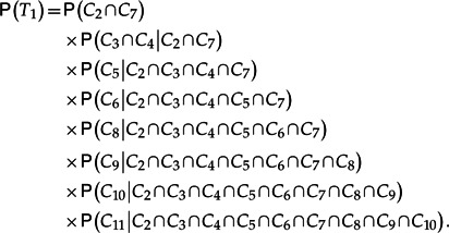
To see how this would work in an example, consider again the tree in Figure 1. By grouping clades with their sister clade when the sister tree is not a single taxon, the exact probability of the tree can be expressed as follows using rules of conditional probability:
 |
(2) |
Under the principle of conditional independence of separated subtrees, most of these conditional probabilities can be greatly simplified. For example, the edge that separates C5 from the rest of the tree separates C6 from all other clades in the tree, so given C5, C6 is approximately independent of all other clades. It follows from the assumption of approximate conditional independence that P(C6|C2 ∩ C3 ∩ C4 ∩ C5 ∩ C7) ≈ P(C6|C5) may be an accurate approximation. Applying this principle of approximate conditional independence to each conditional probability results in the expression
 |
(3) |
To apply this approximation requires a more detailed summary of the tree sample than simply the clade proportions. For example, to estimate P(C6|C5)= P(C5∩C6)/P(C5) from the sample, we need to compute the proportion of trees that include the snow leopard/leopard/tiger clade C5 that also contain the snow leopard/leopard clade C6. In the given sample, this is 50 827/64 942 ≐ 0.7827. Making similar calculations for all nodes and applying Equation (3), the estimated probability for the tree in Figure 1 based on conditional clade distributions is 0.3419 which is very close to the simple proportion of 0.3393 with which the tree appeared in the sample.
The tree T2 in Figure 2 has a slightly different topology and replaces two of the clades from the tree in Figure 1 (C5 and C10) with two others (X5 and X10). The different topology leads to a different approximating equation
 |
(4) |
Using sample relative frequencies to estimate each of these conditional clade probabilities results in an estimate of 1.1×10⁻⁶ for the probability of tree T2, even though this tree was not sampled. The key is that both the cat-like and dog-like subtrees are probable enough to appear in the sample individually, but are sufficiently unlikely that there is a good chance that they are not sampled together.
Methods
The previous section had different approximating equations for each tree. Each of the approximate conditional probabilities in Equations (3) and (4) is of the form P(left subclade∩right subclade|clade) if one includes subclades with only single taxa. For example, in the approximation of the probability of T1, P(C6|C5) = P(C6 ∩ tiger | C5). In addition, the first factor can be written as P(C2 ∩ C7|C1) as C1 is certain for any tree with these 12 taxa. Additional factors such as P(dog∩gray wolf|C11) for each clade of size 2 in the tree could be included in the product as each has a value of 1 as there is no other way to separate a clade of size 2. With these changes, the approximating equation for each tree contains a factor for each internal node in the tree. A general approximating equation for an arbitrary rooted tree T where each clade C of size 2 or more including the clade that is all taxa in the tree is directly divided into two smaller clades L(C,T) and R(C,T), may be written as follows:
 |
(5) |
This equation is easily extended to trees that contain multifurcations taking the probability of the intersection of all children clades should one wish to consider such trees. In the remainder of this article I will refer to the method of using conditional clade probability distributions by applying Equation (5) to approximate tree probabilities as the conditional clade distribution (CCD) method and using simple sample relative frequencies to estimate tree probabilities as the simple relative frequency (SRF) method.
I note that this equation is similar to the conditional clade probability (CCP) formulas given in Höhna and Drummond (2012). The key difference is that in their formulas, the unnormalized probabilities for each tree are the product over all clades in the tree of the conditional clade probabilities of the form P(clade|parent of clade). In the approach in this article, the probability of each tree is calculated as the product over all parent clades in the tree of the conditional clade probabilities of the form P(all children clades|parent clade).
The approach in Höhna and Drummond (2012) requires computing CCP scores for each possible tree and then renormalizing by dividing these scores by their sum to obtain the estimated probabilities. Because of the need for renormalization, their method is not tractable for trees with many taxa without restricting attention to a small subset of possible trees, and even then are less accurate than the method I present here. In contrast, I show in online Appendix 2 (located at the Dryad data repository, doi:10.5061/dryad.k8n14) that applying Equation (5) to each possible tree leads to a valid probability distribution where the sum of probabilities of all trees is one and no renormalization is necessary. Furthermore, in the method of Höhna and Drummond (2012), there is no theoretical justification under which their approximation would be correct, albeit the approximations are accurate in their limited examples with very small trees. In contrast, the method in this article is based on a principle of conditional independence described in the next section which can be justified from the prior distribution on trees and an approximation to the likelihood calculation on trees. The appendix contains a detailed derivation that shows how the approximate conditional independence of separate subtrees is a consequence of the assumption that in trees that fit the data well, there is little uncertainty in the unobserved sequences at internal nodes in the tree.
In addition, Ronquist et al. (2004) describe a Bayesian supertree method that represents a probability distribution on the space of phylogenetic trees with probabilities associated with specific splits related to parsimony scores. I leave it to others to explore this connection in more depth.
Principle of Conditional Independence
The approximation equation (5) is based on the assumption that clades in different parts of the tree are approximately independent. To specify this condition more explicitly, it is useful to consider unrooted trees. The same concepts apply to any rooted tree by considering the corresponding unrooted tree. Each edge of an unrooted tree T corresponds to a split which partitions the taxa into two sets. Let s be a split in T where the removal of the corresponding edge from T leaves behind rooted subtrees T1 and T2. I say that a split s separates splits s1 and s2 in tree T if s1 corresponds to an edge in T1 and s2 corresponds to an edge in T2, or vice versa. The principle of conditional independence of separated subtrees states that if s separates s1 and s2, then s1 and s2 are approximately independent so that P(s1 ∩ s2|s) ≈ P(s1|s2) P(s2|s) and P(s1|s, s2) ≈ P(s1|s). More generally, if each of the m splits a1,...,am is separated from each of the n splits b1,...,bn by split s in a tree T, then splits a1,...,am are approximately conditionally independent of splits b1,...,bn given s, and the following probability relationships are approximately true:
 |
The following computational algorithm is based on this principle.
Computational Algorithm
In order to apply Equation (5), it is necessary to estimate various clade conditional probabilities from a sample of trees. An algorithm to calculate and store the necessary probabilities efficiently is described in online Appendix 1 but described briefly here. One pass through the sample of trees finds the unique trees and a count of how often each is sampled. In a pass through this summary, two maps are formed. Map 1 (m1) counts for each clade that appears in at least one tree the number of trees that contain the clade (including clades of size 1 and the clade of all taxa, the totals of which equal the sample size). The second map (m2) counts for each clade of size 2 or more and its two direct subclades the number of trees that contain this triple of clades. The algorithm also stores the total number of trees sampled by summing the counts.
Once these two maps are stored, the probability of a tree is estimated by taking the product over clades C of size 2 or more with subclades C1 and C2 the conditional probabilities P(C1 ∩ C2|C) ≈ m2(C,C1,C2)/m1(C). If a tree contains a pair of sister clades that are not in the map (and therefore were unsampled together), its probability is estimated to be 0.
Results
In this section I apply the CCD method to a number of data examples and show excellent agreement between it and the SRF method. I also present mathematical results that show how the CCD method extends to unrooted trees and that prove that the CCD method induces a legitimate probability distribution on the set of possible trees.
Demonstration on Carnivora Example
The carnivora example consists of the cox1 gene for 12 taxa including six dog-like and six cat-like taxa. The sample was taken using MrBayes 3.2 (Ronquist et al. 2012) with the BEAGLE library (Ayres et al. 2012) under the HKY85 likelihood model (Hasegawa et al. 1985) with separate parameters for each codon position and using approximate gamma distributed rates (Yang, 1994) with four rate categories. The total sample size was 1.1 million with the first 100 000 trees discarded as burn in and the remaining million trees subsampled every 10 trees. Examination of trace plots of the log-likelihood and comparisons of split probabilities across independent runs are consistent with good mixing and sufficient burn in. There are 654 729 075 possible unrooted trees with 12 taxa. The sample contains only 229 of these trees. The most probable tree was sampled 33 925 times and 50 trees were sampled only once.
For each of these 229 trees, I calculate the probability of the tree first using the simple sample proportions and second using Equation (5). These 229 points are plotted in Figure 3 using both regular axes and logarithmic axes. There is strong agreement between the two calculations for both trees with relatively high and low probability. The correlation between the calculations is 0.997. The largest absolute difference between the two calculations is about 0.017 where the SRF estimate of the second most probable tree (0.1625) is slightly higher than the CCD estimate (0.1454). The sum of the 229 CCD estimated probabilities is 0.9985 which suggests that only about 0.15% of the total probability is missing from the sample. Figure 3b shows that 50 trees sampled only once have CCD probability estimates ranging from 3×10⁻⁸ to 1.4× 10⁻⁴, the larger probability more than 1000 times larger than the smaller, whereas each of these trees has an SRF probability estimate of 1×10⁻⁵.
Figure 3.

A comparison of SRF and CCP Distribution estimates for the Carnivora example: a) displays probabilities, b) shows the same information on a log–log scale.
Validation
I have shown that the CCD method based on the theoretical assumption of approximate conditional independence of separated subtrees is accurate on a single sample from a single data set. To provide additional evidence that this method is valid, I examine its behavior with repeated samples on the Carnivora data set, on a sample from a uniform distribution over tree space where exact calculations are possible, and for multiple other real data sets.
Carnivora example with repeated samples.—Using the Carnivora data set from the previous section, I added 9 more runs with different streams of random variables using the identical model and MCMC parameters and summarize the 10 total runs. The number of unique trees was 249.7 ±16.2 (mean ± standard deviation) and the estimated proportion of the total tree space covered by each individual sample was 0.9985±0.0002. Over all 10 runs, a total of 470 trees were sampled, so many trees appear in only one or a few samples. The correlation between the SRF and CCD probability estimates for trees sampled in each data set is 0.9970±0.0007, indicating strong agreement between these estimates for each sample. The SRF probabilities of the trees in Figures 1 and 2 are 0.3367 ±0.0092 and 3.00×10⁻⁶ ±4.83×10⁻⁶, respectively, when compared with the CCD probability estimates of 0.3411±0.0094 and 1.23×10⁻⁶ ±4.49×10⁻⁷. The CCD probability estimate of Figure 1 tree is slightly larger than the SRF estimate in each of the 10 DSs (0.0045±0.0029), which confirms that there is some bias in the CCD probability estimation of the true distribution. However, the sample to sample variability is about the same for both estimation methods and at this MCMC sample size, the size of the approximation bias is smaller than the standard deviation due to sampling variation for the most probable tree. Note that the SRF estimates of the tree in Figure 2 are based on three estimates of 1/100 000 and 7 of 0. For the low probability tree in Figure 2, the CCD probability estimates are substantially less variable. This suggests that using the CCD method introduces only a small amount of bias at little penalty in variance when estimating probabilities of highly probable trees, but greatly reduces the variance in estimating probabilities of more unlikely trees.
Figure 4a displays the relative standard deviations (standard deviation divided by the mean of the SRF estimates) of the CCD estimates versus the SRF estimates across the 10 samples for each of the 470 trees found in at least one sample. The line is drawn where these values are equal. Most of the points fall below the line, which means there is less sample to sample variation for the CCD method than the SRF method for almost all trees for this data set. This is consistent with the idea that clade probability estimates are estimated with less variation from samples than are tree probabilities. Thus, the approximations based on CCDs are much less variable from sample to sample for most of the trees with nonnegligible probability. The line of points to the right of 3 on the horizontal axis are from the trees sampled once in one sample and not at all in other samples.
Figure 4.

Variation in estimates for the Carnivora example. a) The quantity on the x-axis is the standard deviation of the 10 SRF estimates from different MCMC samples divided by the mean of the same values. The quantity on the y-axis is the standard deviation of the 10 CCD estimates divided by the mean of the 10 SRF estimates. b) The quantity on the x-axis is the base 10 logarithm of the mean SRF estimates. The quantity on the y-axis is the absolute value of the difference in the mean CCD and SRF estimates divided by the standard deviation of the SRF estimates, also on a logarithmic scale.
Figure 4b plots the ratio of the absolute mean difference in the two estimates to the standard deviation of the SRF estimates against means of the SRF estimates for all trees sampled at least once with both variables plotted on a log scale to spread out the points near the origin. This display shows that the size of the absolute bias is smaller than the standard deviation of the SRF estimates for the majority of the trees. A large majority of the points fall below the dotted line at zero where the absolute bias due to the approximation is less than the size of the uncertainty due to sampling variability. The positive trend in this plot indicates that the size of the potential estimation bias relative to the size of the error due to sample to sample uncertainty tends to be smaller for very low probability trees than for more probable trees.
To summarize, replacing simple estimates with conditional clade probability estimates introduces a small amount of bias for each tree. However, the size of this bias is fairly small and often may be smaller than the MCMC uncertainty of the simple estimates from a single MCMC sample. For less probable trees in particular, the conditional clade probability estimates from a single sample are likely both more accurate and less variable than simple estimates from a single sample, at least for this single data set.
Samples from a uniform distribution.—To explore the behavior of the CCD method in a case where the probability distribution is diffuse and the true probabilities are known exactly, I took an independent sample of 100 000 trees from a uniform prior distribution on the space of unrooted trees with 10 taxa, of which there are 2 027 025. This sample size was large enough to estimate the clade distributions well, but too small for the SRF method to be accurate. Each tree has true probability about 4.9×10⁻⁷, but a tree sampled once will have SRF probability of 1.0×10⁻⁵ and some multiple of this if it is sampled multiple times. There were 97 722 unique trees included in the sample, one of which was sampled four times. The SRF probability estimates for each of these trees is far larger than the true probability. In contrast, the CCD probability estimates for these sampled trees vary from 6×10⁻⁸ to 1.6×10⁻⁶ and the median estimate is 5.2×10⁻⁷ which is very close to the true value. The estimate of the total coverage of the sample (sum of all approximate probabilities) is 0.0524 which is close to the correct value of 97 722/2.027.025 ≐ 0.04821.
To further explore the accuracy of the CCD approximation of this true uniform distribution, I took a second random sample of 100 000 trees and used the estimated conditional clade distributions from the first sample to estimate probabilities of trees in the second sample. The second sample had 97 516 unique trees, only about 5% of which were also in the first sample. The estimated probabilities of these trees ranged from 0 to 1.6×10⁻⁶ and the median estimated probability was 4.8×10⁻⁷, very close to the true value of 4.9×10⁻⁷. Only 36 of these trees had estimated probabilities of zero based on the conditional clade distributions of the first sample; the lowest estimated probability for those for which it was positive was 5×10⁻⁸. The mean and standard deviation of the CCD estimated probabilities was 4.9×10⁻⁷ ±1.5×10⁻⁷ and was centered over the true value. The sum of estimated probabilities of trees in this second sample is 0.0480, very close to the true value of 97 516/2 027 025 ≐ 0.0481.
This example shows that the CCD estimates can be very accurate, even when applied to trees that are not in the original sample. In this instance where the true probability of the most probable tree is substantially less than the reciprocal of the sample size, the CCD estimates are much more accurate and less variable from sample to sample than are the SRF estimates.
A much larger data set.—Poux et al. (2006) constructed and analyzed a data set using three unrelated genes from 62 mammalian taxa that included two marsupial outgroups, representatives of all extant placental mammalian orders, and heavy representation of South American rodents and primates, the primary foci of the study. I used a much simpler model than the authors and treated all 3768 sites in the alignment identically using the general time reversible (GTR) model (Tavaré, 1986) with approximate gamma distributed rates using four rate categories.
Using MrBayes 3.2 with the BEAGLE library I ran MCMC for 5 500 000 generations, discarded the first 500 000 as burn in, and subsampled every 100th tree, resulting in a sample of 50 000 trees. Comparisons split probability estimates with a second run of the same size support the conclusions that the size of this sample was sufficiently large and that the chain mixed well (data not shown). Figure 5 shows a graph of the simple and conditional clade estimates of the probabilities of each of the 4297 sampled trees. The correlation between these two measures is 0.990. The sum of the conditional clade probability estimates is 0.9150, so this sample likely represents over 90% of the total probability, but about 8.5% of the probability resides on unsampled trees. The largest absolute difference between the two estimates is 0.008. The most probable tree has SRF estimate 0.0655 and CCD estimate 0.0604. This example demonstrates that the CCD method can be accurate even when tree space is enormous; there are about 6.97 ×1098 unrooted trees with 62 taxa, much greater than the estimated 1080 atoms in the observable universe. A sample of 50 000 trees cannot estimate all of these probabilities accurately, but the CCD method provides a means to estimate accurately the probabilities of the sampled trees and for many relatively probable trees not included in the sample.
Figure 5.

SRF and CCD comparison in the 62-taxon mammalian example.
Additional data sets.—Lakner et al. (2008) and Höhna and Drummond (2012) examine the performance of many MCMC sampling procedures across 11 DSs with various numbers of taxa and nucleotide sites. Further details about these data sets are included in these papers and in Table 2. For each of these data sets, I used MrBayes 3.2 with the BEAGLE library treating all sites as identically distributed with the GTR model with approximate gamma distributed rates using four rate categories to sample 5 500 000 trees, discarding the first 500 000 as burn in and subsampling each 50th tree of the remainder for a sample of 100 000 trees from each data set. The results are summarized in Table 3. A second set of runs under the same conditions, but with different random numbers, shows very similar results, indicating that these MCMC samples are likely not to suffer from poor convergence (data not shown).
Table 2.
Eleven additional DSs
| Data set | # Taxa | # Sites | Legacy TreeBASE | Current TreeBASE | Tree space size |
|---|---|---|---|---|---|
| DS 1 | 27 | 1949 | M336 | M2017 | 5.84×1031 |
| DS 2 | 29 | 2520 | M501 | M2131 | 1.58×1035 |
| DS 3 | 36 | 1812 | M1510 | M127 | 4.89×1047 |
| DS 4 | 41 | 1137 | M1366 | M487 | 1.01×1057 |
| DS 5 | 50 | 378 | M3475 | M2907 | 2.84×1074 |
| DS 6 | 50 | 1133 | M1044 | M220 | 2.84×1074 |
| DS 7 | 59 | 1824 | M1809 | M2449 | 4.36×1092 |
| DS 8 | 64 | 1008 | M755 | M2261 | 1.04×10103 |
| DS 9 | 67 | 955 | M1748 | M2389 | 2.13×10109 |
| DS 10 | 67 | 1098 | M520 | M2152 | 2.13×10109 |
| DS 11 | 71 | 1082 | M767 | M2274 | 6.85×10117 |
Table 3.
Results from 11 additional DSs
| Data set | Sampled treesa | Coverageb | Corr.c | Max. abs. diff.d | Max CCDe | Max SRFf |
|---|---|---|---|---|---|---|
| DS 1 | 8333 | 0.654 | 0.777 | 0.02760 | 0.01741 | 0.04407 |
| DS 2 | 3473 | 0.979 | 0.973 | 0.00979 | 0.03857 | 0.03707 |
| DS 3 | 2861 | 0.984 | 0.995 | 0.01601 | 0.17888 | 0.16880 |
| DS 4 | 18 680 | 0.683 | 0.867 | 0.00598 | 0.00762 | 0.00930 |
| DS 5 | 96 608 | 7.45×10⁻⁵ | 0.047 | 0.00004 | 5.64×10⁻⁷ | 0.00004 |
| DS 6 | 81 218 | 0.187 | 0.606 | 0.00010 | 0.00014 | 0.00015 |
| DS 7 | 30 537 | 0.749 | 0.972 | 0.00034 | 0.00245 | 0.00241 |
| DS 8 | 84 629 | 0.021 | 0.273 | 0.00010 | 0.00005 | 0.00013 |
| DS 9 | 99 209 | 3.70×10⁻¹² | 0.006 | 0.00003 | 1.18×10⁻¹³ | 0.00003 |
| DS 10 | 89 811 | 1.23×10⁻³ | 0.066 | 0.00006 | 3.61×10⁻⁶ | 0.00006 |
| DS 11 | 99 791 | 1.40×10⁻¹⁵ | 0.0003 | 0.00002 | 1.18×10⁻¹⁶ | 0.00002 |
aNumber of distinct trees in the sample.
bSum of CCD estimated probabilities in the sample.
cCorrelation between CCD and SRF estimates.
dMaximum absolute difference between CCD and SRF estimates.
eMaximum CCD estimate for trees in the sample.
f Maximum SRF estimate for trees in the sample.
The comparisons between the SRF and CCD methods vary across these data sets. I will discuss the results separately for groups of data sets for which the behavior is somewhat similar.
DS 2, DS 3, and DS 7 are somewhat similar to the 62-taxon mammal DS from the previous section in that the sample of trees contains a large fraction of the total posterior distribution (about 75% or higher) and the correlation between the CCD and SRF estimates of tree probabilities within the sample is greater than 0.97. There is generally very strong agreement between the estimates, as seen in Figure 6b for DS 2.
Figure 6.

Comparison between SRF and CCD estimates in some additional DSs. a) DS 1; b) DS 2; c) DS 4; d) DS 6; e) DS 8; and f) DS 10.
DS 1 and DS 4 have estimated coverage between 60% and 70% and lower correlations between the estimates (0.777 and 0.606). In these two DSs, there is a fair amount of variation in the CCD estimates among the many trees with relatively low SRF estimates, which lowers the correlation between these measures when compared with the data sets with larger coverage. In addition, DS 1 has some quirks where there are several trees that are sampled only once, but have CCD estimates much larger than 1 in 100 000. Many of the points are below the line in Figures 6a and c due to the fact that the coverage is substantially below 1.
DS 6 and DS 8 have coverage between 2% and 20%, maximal SRF estimates between 0.0001 and 0.0002 as no trees are sampled more than 20 times out of 100 000, and maximal CCD estimates about the same. There is significant positive correlation between the two methods for computing tree probabilities, but the association is weaker than the previous examples because the SRF method simply does not discriminate much among the sampled trees. In contrast, the CCD method varies over several orders of magnitude among trees sampled the same number of times and is measuring the posterior probabilities of these trees much more precisely.
The total coverage of the sample according to CCD for DS 5, DS 9, DS 10, and DS 11 is estimated to be much less than 1%. In these cases, the posterior distribution is very diffuse and even the most probable trees individually have very low probabilities. In some cases, the coverage is less by many orders of magnitude. For example, in DS 9 and DS 11, the coverage of the entire samples is estimated by the CCD method to be on the order of 10−12 and 10−15, far smaller than the 10−5 estimated probability for almost all single trees using the SRF method. Figure 6f shows the comparison between SRF and CCD estimates for DS 10. The CCD estimates are close to zero for nearly all trees and are not substantially higher for trees sampled more than once compared with those sampled only once. Consequently, the correlation between the measures is nearly zero. This reflects that the SRF estimates are quite inaccurate and highly variable. In fact, for DS 11, a second random sample contains 99 790 distinct trees, none of which are in the first sample. For this data set, samples of more than 1016 trees would be required for even the most probable trees to be sampled with high probability more than a few times. Clearly, when the posterior distribution is so diffuse that even the most probable trees have smaller probability than one over the sample size, the SRF estimates of tree probabilities are far too large for trees in the sample. However, clade and conditional clade probabilities can be estimated more accurately and the CCD method provides a means to approximate tree probabilities from these distributions.
To further illustrate this point, DS 11 contains 71 taxa, and the true unrooted tree will have 68 nontrivial splits (those that do not separate just a single taxon from the rest). In the single MCMC sample of 100 000 trees, there were 21 splits with probability greater than 0.99, 29 with probability greater than 0.9, and 40 with probability greater than 0.5. The majority rule consensus tree has a fair amount of resolution, even though a lot of uncertainty remains in the tree. Many additional splits are probable enough that trees that contain them appear many times in the sample. The probabilities of these splits can be estimated with relatively small sampling error and the CCD method uses these accurate clade probability estimates to produce accurate tree probabilities when the SRF method fails.
To summarize, in cases where the MCMC sample represents a substantial fraction of the total posterior distribution, there is strong agreement between SRF and CCD estimates of tree probabilities. In cases where the coverage is low, SRF estimates for individual trees are unreliable, and so correlations between SRF and CCD estimates are weak.
Some Mathematical Results
I have presented the CCD method for estimating tree probabilities from conditional clade distributions on the basis of an assumption of approximate conditional independence among clades in separated subtrees and have shown close agreement between these estimates and SRF estimates when MCMC samples are large enough for SRF estimates to be accurate for many data sets. I justified the method with an appeal to a property on unrooted trees, but described the computational algorithm with regard to rooted trees. In addition, I have made other statements about mathematical properties of the CCD method without justification. The following list summarizes mathematical results about the CCD method for estimating tree probabilities. The rigorous mathematical arguments to support these results are described in online Appendix 2.
The CCD method for estimating tree probabilities of unrooted trees is invariant to different rootings of the trees.
- The computational method in Equation (5) for rooted trees is equivalent to the following expression for unrooted trees:
where the node n is incident to 3 edges that correspond to the splits s1(n), s2(n), and s3(n).
(6) For any full specification of CCP distributions, the sum of the corresponding probabilities in Equation (5) taken over all possible rooted trees for the given set of taxa equals 1; hence, the CCD method defines a valid probability distribution on the set of all possible trees.
A derivation of the result that approximate conditional independence of separated subtrees follows from the form of the calculation of the likelihood in phylogenetic models is shown in online Appendix 3. A theoretical argument that smaller samples are needed to estimate probability distributions on trees that follow the conditional independence of separated subtree principle than to estimate general tree distributions is described in online Appendix 4.
Software
I have written C++ code that implements the concepts of this article. The code is available currently on my web site for download under the name ccd-probs (Larget, 2012) and is available at sourceforge.net/projects/ccdprobs. The software runs from a command line interface and includes separate components to: (i) summarize raw MrBayes output files with the mbsum program from Larget et al. (2010) and (ii) apply the CCD method to estimate the probabilities of all sample trees. The program creates an additional output file with the single split and joint triple split maps that can in principle be read by other programs that wish to apply the CCD probability distribution from a given set of trees without reprocessing the sample summaries. In addition, the program can take as input a second file of trees that are not part of the data for forming the maps, but whose probability can also be evaluated. The software uses the dynamic bitset functionality of the BOOST C++ library (Siek and Allison, 2012) to efficiently store clades.
Discussion
The estimation of tree posterior probabilities by their SRFs in MCMC samples treats all possible trees as equivalent and ignores the underlying relatedness among trees due to shared clades. Especially in situations where posterior distributions on trees are diffuse and MCMC sample sizes are small relative to the size of the set of trees that contain a high proportion of the posterior probability, information from CCDs helps to smooth the estimation of the full posterior distribution by spreading probability from sampled trees to unsampled trees that contain probable clades. This statistical smoothing of estimated tree probabilities can be important in some applications of Bayesian phylogenetics.
Ramifications
Interpretations of consensus trees.—The results in this article will not drastically change the basic interpretations found in typical Bayesian phylogenetic analyses, but do offer modest improvements. Authors usually summarize a Bayesian posterior distribution on trees by reporting a consensus tree of the sample and annotating edges in this tree with posterior probabilities. This tree is simply a graphical way to display the collection of most probable clades, and one point of this article is to state that these clade probabilities are generally estimated accurately in MCMC samples, even when the probabilities of specific trees may not be. The CCD method in the article, however, will provide users of Bayesian phylogenetic methods a new tool for assessing how thoroughly their MCMC sample covers tree space by calculating the sum of CCD probabilities over all sampled trees. Particularly when there are many taxa, there can be large differences from data set to data set in how diffuse the posterior distribution is. I am not aware of any previous methods that allow one to estimate the fraction of the posterior distribution represented by the posterior sample in Bayesian phylogenetics. The ability to calculate this coverage may improve interpretations of results of Bayesian analyses. Some authors summarize posterior distributions by reporting the number of trees in the sample needed to obtain a high percentage, such as 90, 95, or 99, of the posterior sample. The work in this article shows that in many instances, the number of trees needed to include a high percentage of the sample may be a gross underestimate of the number of trees needed to cover the same percentage in the true posterior distribution.
Note that the previous statement does not imply that MCMC samples with low coverage have mixed poorly or lead to poor inferences. Small samples can lead to accurate estimates. Furthermore, most interesting phylogenetic hypotheses relate to clades and not to the complete specification of the tree. Even when there is significant uncertainty in the complete specification of the tree, there is often strong information about the posterior probability of many clades.
In addition, note that the notion of coverage introduced in this article (the total posterior probability of all sampled trees) is distinct from the frequentist notion of “coverage probability” (the probability that a confidence interval contains the true value of a parameter).
Potential improvements in BEAST.—Höhna and Drummond (2012) created their CCP method for estimating tree probabilities from conditional clade distributions in order to speed up the mixing rate of MCMC proposal distributions and implemented the method in BEAST. The idea is that an initial standard MCMC run can be performed in order to estimate conditional clade probabilities and these probabilities can then be used by subsequent proposal methods to propose new trees from a distribution close to the true posterior distribution rather than uniformly at random like many currently implemented MCMC proposal methods. The CCD method in this article does not require renormalization, and thus ought to be substantially faster. In addition, the assumption of conditional independence among separated subtrees appears to be reasonably benign in real data sets which suggests that the CCD method may come closer than the CCP method of Höhna and Drummond (2012) to accurately estimate true posterior distributions. I have not tested either of these claims rigorously; the speed claim appears self-evident because the calculations require nearly identical work up to renormalization, and the renormalization step of the CCP method is the most time-consuming step by far. The only evidence I have that the CCD method is more accurate than the CCP method for estimating tree probabilities is that the CCD method will be exactly correct under the reasonable approximating assumption of conditional independence in separated subtrees and the CCP method is based on no such theory. In addition, after renormalization, the CCP method will place a total probability of one on the set of all trees it considers. For many data sets, the true sum of these probabilities can be much smaller than one when the set of trees is small relative to the size of tree space. It is possible that replacing algorithms in BEAST that use their CCP method with an algorithm based on the CCD method in this article will improve the efficiency of MCMC sampling in this program. Similar ideas could be implemented in MrBayes.
A new class of importance sampling algorithms.—In conjunction with a method to propose branch lengths given a tree topology, the CCD method of this article could be used to generate trees at random from a distribution that mimics the true posterior distribution after an initial calculation to estimate conditional clade distributions. Independent samples from this proposal distribution could be used as the basis for importance sampling from the posterior distribution. If the CCD-based proposal distribution is an accurate enough representation of the true posterior distribution, importance sampling could replace MCMC and allow for independent samples from the posterior to be taken efficiently. Note that MCMC would still be required to set up the conditional clade probability distributions. Much work remains to develop these rough ideas into practical algorithms and tested software, but there is the distinct possibility that CCD-based importance sampling could greatly speed up Bayesian sampling from posterior distributions on phylogenetic trees, allowing for significant computational time savings for large data sets.
Improved accuracy in BCA.—BCA is sensitive to the estimation of small tree probabilities from data in some genes when those trees are highly probable in other genes. The CCD method in this article can be used to improve the accuracy of BCA in measuring the probability of discordance among gene trees by providing a means to estimate the probabilities of unsampled trees.
Alternative sampling methods for large trees.—If the assumption of conditional independence among separated subtrees is not too inaccurate, this suggests that Bayesian analysis of large trees could begin by partitioning taxa into groups that are likely to be separated on the true tree, carrying out separate analyses for these groups, and combining the results under the assumption of conditional independence. The computational effort of analyzing multiple data sets with smaller taxon sets lends itself to parallel computing and speedups due simply to working on smaller subtrees. For example, for the Carnivora data set from the beginning of the aricle (or a larger similar example), it could be possible to run separate analyses for the cat-like and dog-like taxa, perhaps with a few cross representatives each and then combine the results to obtain a sample from the larger tree space. A great deal of work is required to explore the potential gains in computational efficiency and to protect against bias from the conditional independence approximation. However, the good fit between true distributions and approximations that assume conditional independence suggests that some sort of the divide and conquer approach for large trees may work well without introducing too much bias.
Summary
The CCD method for estimating tree probabilities from CCDs solves a long-standing problem among developers of phylogenetic methods on how to use clade information to better estimate probabilities of trees. The method provides a new tool to augment standard Bayesian phylogenetic analyses by allowing the scientist to estimate the proportion of tree space covered by the MCMC sample. The method will patch a hole in BCA when implemented in the program BUCKy. More importantly, the method has the potential, when further developed and combined with other ideas, to lead to new computational approaches for Bayesian phylogenetic inference that could be substantially more efficient than the current state of the art.
Supplementary Material
Supplementary material, including data files and online-only appendices, can be found in the Dryad data repository at http://datadryad.org, doi:10.5061/dryad.k8n14.
Funding
This work was supported by the National Institutes of Health [grant number 1 R01 GM086887]; and the National Science Foundation [DEB 0949121, DEB 0936214].
Acknowledgments
The author thanks Cécile Ané for countless helpful discussions about the research in this article. The author thanks all three referees and the associate editor for helpful suggestions that improved the final paper. In particular, the author thanks Alexei Drummond for the basis of the calculations for comparing the number of free parameters in probability distributions on general tree spaces and on those that obey the principle of conditional independence of subtrees that is in online Appendix 4.
References
- Ané C., Larget B., Baum D.A., Smith S.D., Rokas A. Bayesian Estimation of Concordance among Gene Trees. Mol. Biol. Evol. 2007;24:412–426. doi: 10.1093/molbev/msl170. [DOI] [PubMed] [Google Scholar]
- Arnason U., Gullberg A., Janke A., Kullberg M., Lehman N., Petrov E.A., Vainola R. Pinniped phylogeny and a new hypothesis for their origin and dispersal. Mol. Phylogenet. Evol. 2006;41:345–354. doi: 10.1016/j.ympev.2006.05.022. [DOI] [PubMed] [Google Scholar]
- Ayres D.L., Darling A., Zwickl D.J., Beerli P., Holder M.T., Lewis P., Huelsenbeck J.P., Ronquist F., Swofford D.L., Cummings M.P., Rambaut A., Suchard M.A. Beagle: an application programming interface for statistical phylogenetics. Syst. Biol. 2012;61:170–173. doi: 10.1093/sysbio/syr100. [DOI] [PMC free article] [PubMed] [Google Scholar]
- Bjornerfeldt S., Webster M.T., Vila C. Relaxation of selective constraint on dog mitochondrial DNA following domestication. Genome Res. 2006;16:990–994. doi: 10.1101/gr.5117706. [DOI] [PMC free article] [PubMed] [Google Scholar]
- Burger P., Steinborn R., Walzer C., Petit T., Mueller M., Schwarzenberger F. Analysis of the mitochondrial genome of cheetahs (Acinonyx jubatus) with neurodegenerative disease. Gene. 2004;338:111–119. doi: 10.1016/j.gene.2004.05.020. [DOI] [PMC free article] [PubMed] [Google Scholar]
- Drummond A.J., Rambaut A. BEAST: Bayesian evolutionary analysis by sampling trees. BMC Evol. Biol. 2007;7:214. doi: 10.1186/1471-2148-7-214. [DOI] [PMC free article] [PubMed] [Google Scholar]
- Hasegawa M., Kishino H., Yano T. Dating the human-ape split by a molecular clock of mitochondrial DNA. J. Mol. Evol. 1985;22:160–174. doi: 10.1007/BF02101694. [DOI] [PubMed] [Google Scholar]
- Höhna S., Drummond A.J. Guided Tree Topology Proposals for Bayesian Phylogenetic Inference. Syst. Biol. 2012;61:1–11. doi: 10.1093/sysbio/syr074. [DOI] [PubMed] [Google Scholar]
- Holder M.T., Sukumaran J., Lewis P.O. A justification for reporting majority-rule consensus tree in Bayesian phylogenetics. Syst. Biol. 2008;57:814–821. doi: 10.1080/10635150802422308. [DOI] [PubMed] [Google Scholar]
- Huelsenbeck J., Ronquist F. MrBayes: Bayesian inference of phylogeny. Bioinformatics. 2001;17:754–755. doi: 10.1093/bioinformatics/17.8.754. [DOI] [PubMed] [Google Scholar]
- Kim K.S., Lee S.E., Jeong H.W., Ha J.H. The complete nucleotide sequence of the domestic dog (Canis familiaris) mitochondrial genome. Mol. Phylogenet. Evol. 1998;10:210–220. doi: 10.1006/mpev.1998.0513. [DOI] [PubMed] [Google Scholar]
- Lakner C., van der Mark P., Huelsenbeck J.P., Larget B., Ronquist F. Efficiency of Markov chain Monte Carlo tree proposals in Bayesian phylogenetics. Syst. Biol. 2008;57:86–103. doi: 10.1080/10635150801886156. [DOI] [PubMed] [Google Scholar]
- Larget B. 2012. CCDprob: software for estimating tree probabilities from conditional clade distributions. Available from: URL http://www.stat.wisc.edu/~larget/ccd/ (last accessed March 13, 2013) [Google Scholar]
- Larget B., Kotha S.K., Dewey C.N., Ané C. BUCKy: gene tree/species tree reconciliation with the Bayesian concordance analysis. Bioinformatics. 2010;26:2910–2911. doi: 10.1093/bioinformatics/btq539. [DOI] [PubMed] [Google Scholar]
- Lopez J.V., Cevario S., O'Brien S.J. Complete nucleotide sequences of the domestic cat (Felis catus) mitochondrial genome and a transposed mtDNA tandem repeat (Numt) in the nuclear genome. Genomics. 1996;33:229–246. doi: 10.1006/geno.1996.0188. [DOI] [PubMed] [Google Scholar]
- Poux C., Chevret P., Huchon D., de Jong W.W., Douzery E.J.P. Arrival and diversification of caviomorph rodents and platyrrhine primates in South America. Syst. Biol. 2006;55:228–244. doi: 10.1080/10635150500481390. [DOI] [PubMed] [Google Scholar]
- Ronquist F., Huelsenbeck J.P. MrBayes 3: Bayesian phylogenetic inference under mixed models. Bioinformatics. 2003;19:1572–1574. doi: 10.1093/bioinformatics/btg180. [DOI] [PubMed] [Google Scholar]
- Ronquist F., Huelsenbeck J.P., Britton T. Bayesian Supertrees. In: Bininda-Emonds O.R., editor. Phylogenetic supertrees: combining information to reveal the tree of life, Vol. 3. Alphen aan den Rijn (The Netherlands): Kluwer Academic; 2004. pp. 193–224. [Google Scholar]
- Ronquist F., Teslenko M., van der Mark P., Ayres D.L., Darling A., Höhna S., Larget B., Liu L., Suchard M.A., Huelsenbeck J.P. MrBayes 3.2: efficient Bayesian phylogenetic inference and model choice across a large model space. Syst. Biol. 2012;61:539–542. doi: 10.1093/sysbio/sys029. [DOI] [PMC free article] [PubMed] [Google Scholar]
- Siek J., Allison C. 2012. Boost Dynamic Bitset Library. Available from: URL http://www.boost.org/ [Google Scholar]
- Tavaré S. Some probabilistic and statistical problems on the analysis of DNA sequences. Lect. Math. Life Sci. 1986;17:57–86. [Google Scholar]
- Wei L., Wu X., Jiang Z. The complete mitochondrial genome structure of snow leopard panthera uncia. Mol. Biol. Rep. 2009;36:871–878. doi: 10.1007/s11033-008-9257-9. [DOI] [PubMed] [Google Scholar]
- Wei L., Wu X., Zhu L., Jiang Z. Mitogenomic analysis of the genus panthera. Sci. China Life Sci. 2011;54:917–930. doi: 10.1007/s11427-011-4219-1. [DOI] [PubMed] [Google Scholar]
- Wu X., Zheng T., Jiang Z., Wei L. The mitochondrial genome structure of the clouded leopard (Neofelis nebulosa) Genome. 2007;50:252–257. doi: 10.1139/g06-143. [DOI] [PubMed] [Google Scholar]
- Yang Z. Maximum likelihood phylogenetic estimation from DNA sequences with variable rates over sites: approximate methods. J. Mol. Evol. 1994;39:306–314. doi: 10.1007/BF00160154. [DOI] [PubMed] [Google Scholar]